Matrix multiplication is defined for two matrices when the number of columns in the first matrix equals the number of rows in the second matrix. For example, if matrix (A) has dimensions (m x k), then matrix (B) must have dimensions (k x n) for the multiplication to be valid. The resulting matrix (C) will have dimensions (m x n).
Each element of (C) is computed as the sum of the products of corresponding elements from a row of (A) and a column of (B). In other words, the value at position C[i][j] is obtained by multiplying each element of the i-th row of (A) with the corresponding element of the j-th column of (B), and then summing the results.
Understanding matmul kernel
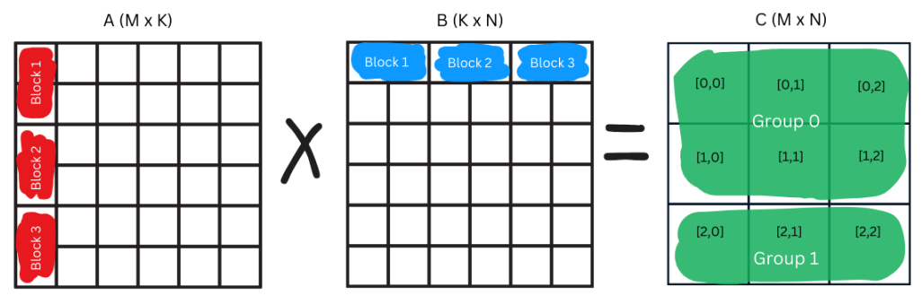
Suppose we have matrix A with dimension (M x K) and matrix B with dimension (K X N) then our resulting matrix C has dimension (M x N).
@triton.jitdef matmul_kernel(# Pointers to matrices a_ptr, b_ptr, c_ptr,# Matrix dimensions M, N, K,# The stride variables represent how much to increase the ptr by when moving by 1# element in a particular dimension. E.g. `stride_am` is how much to increase `a_ptr`# by to get the element one row down (A has M rows). stride_am, stride_ak, # stride_bk, stride_bn, # stride_cm, stride_cn,# Meta-parameters BLOCK_SIZE_M: tl.constexpr, BLOCK_SIZE_N: tl.constexpr, BLOCK_SIZE_K: tl.constexpr, # GROUP_SIZE_M: tl.constexpr, # ACTIVATION: tl.constexpr #):
  Cell In[1], line 17
    ):
      ^
SyntaxError: incomplete input
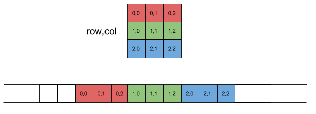
The @triton.jit decorator in Triton is used to compile a Python function as a Triton kernel allowing it to be executed efficiently in GPU. The a_ptr, b_ptr and c_ptr are the pointers to matrices A, B and C respectively. These contain the starting memory address in GPU global memory for the matrix i.e. a_ptr contains the memory address for A[0][0]. In GPU, matrices are stored in row-major order, which means that every elemets of our 2D matrix are stored in 1D memory layout. So for this reason we require stride to get next row element or column element of our matrix. stride_am represents number of elements in 1D memory layout to skip so that we obtain the element of our next row in matrix A and similarly stride_ak represents number of elements in 1D memory layout to skip so that we obtain the element of our next column in matrix A, which is usually 1.
2D row-major memory layout
The BLOCK_SIZE_M, BLOCK_SIZE_N and BLOCK_SIZE_K are the size of our block along those axises. GROUP_SIZE_M is the maximum number of rows per group.
L2 Cache optimization
# -----------------------------------------------------------# Map program ids `pid` to the block of C it should compute.# This is done in a grouped ordering to promote L2 data reuse.# See above `L2 Cache Optimizations` section for details. pid = tl.program_id(axis=0) num_pid_m = tl.cdiv(M, BLOCK_SIZE_M) num_pid_n = tl.cdiv(N, BLOCK_SIZE_N) num_pid_in_group = GROUP_SIZE_M * num_pid_n group_id = pid // num_pid_in_group first_pid_m = group_id * GROUP_SIZE_M group_size_m =min(num_pid_m - first_pid_m, GROUP_SIZE_M) pid_m = first_pid_m + ((pid % num_pid_in_group) % group_size_m) pid_n = (pid % num_pid_in_group) // group_size_m
The num_pid_m is the number of blocks in the M axis and num_pid_n is the number of blocks in the N axis. Suppose N = 384 and BLOCK_SIZE_N = 128 then num_pid_n = ceil(384/128) = 3 i.e. there are 3 blocks in a row. Let’s consider GROUP_SIZE_M = 2 then num_pid_in_group = 2 * 3 = 6 i.e a group in our C matrix contains 6 program ids (each block is 1 pid). For a given program id we can find the group in which it belongs to by group_id = pid // num_pid_in_group. Then we calculate the starting row index in matrix A and C for the current group of thread blocks using first_pid_m = group_id * GROUP_SIZE_M.
Instead of processing an entire matrix at once, we break our matrix into blocks. Each block fits into to the L1 cache.
Blocks and group
The group_size_m is a runtime variable that calculates the actual number of rows a group processes, since there can be edge cases when total rows is less then GROUP_SIZE_M. The example table below shows the calculation of pid_m and pid_n for num_pid_m = 3, num_pid_n = 3, and GROUP_SIZE_M = 2. This grouping strategy is used to optimize L2 cache usage by having nearby threads work on blocks that share data.
pid
group_id
pid_m
pid_n
0
0
0
0
1
0
1
0
2
0
0
1
3
0
1
1
4
0
0
2
5
0
1
2
6
1
2
0
7
1
2
1
8
1
2
2
Threads (pid) in same group work on contiguous rows of the output matrix. For example: * pid=0 to pid=5 work on rows 0 and 1 of the output matrix. * pid=6 to pid=8 work on row 2.
This means that threads in the same group access nearby memory locations in the input matrices (A and B), which improves spatial locality. When one thread loads a block of data into the L2 cache, nearby threads can reuse that data, reducing the number of global memory accesses. Without grouping, threads might access disjoint regions of memory, causing frequent cache thrashing. Grouping ensures that threads in the same group access overlapping or nearby regions, reducing cache thrashing. Or simply, threads within a group compute blocks of C that are close to each other in memory, improving L2 cache utilization.
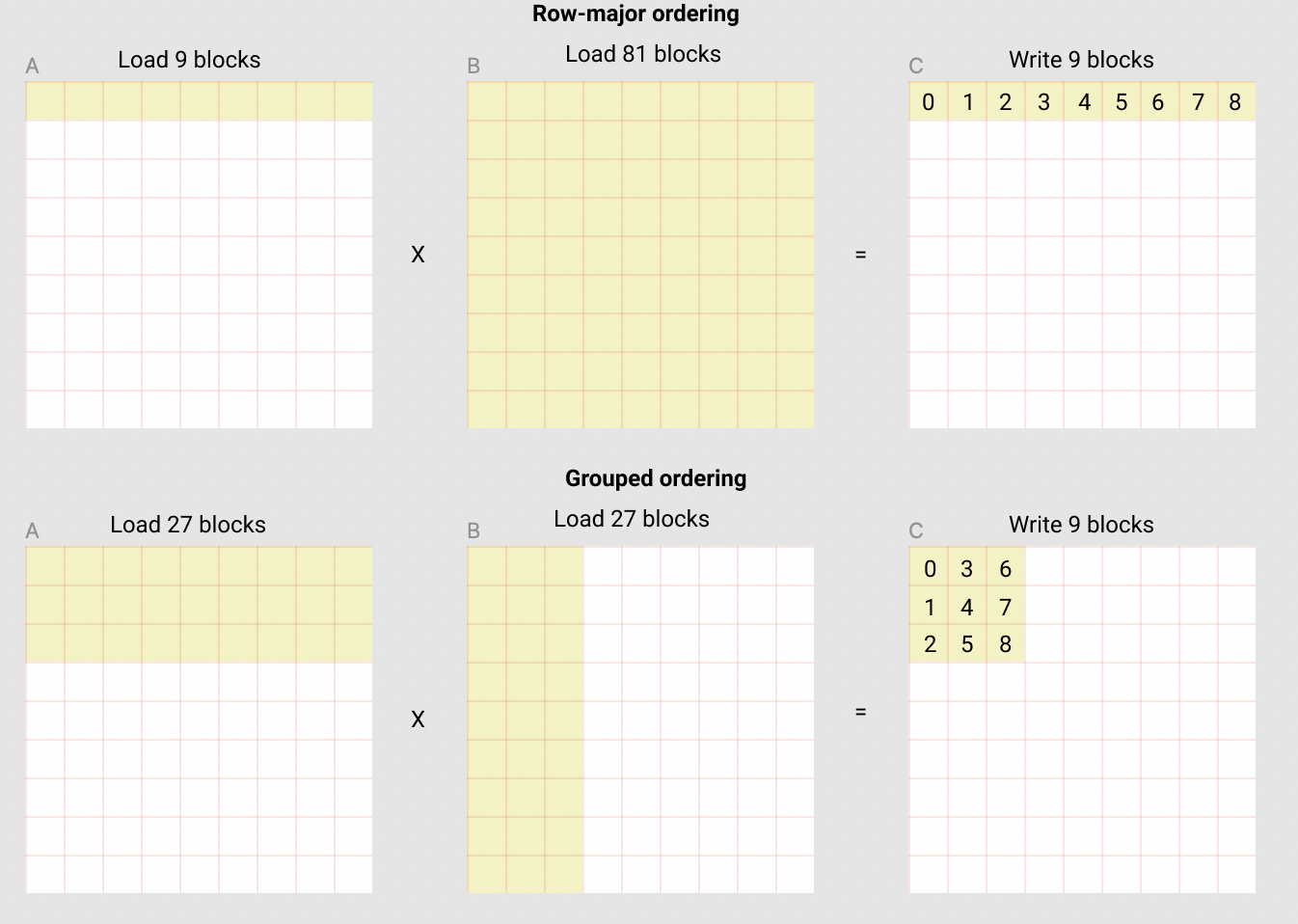
Calculating our output matrix in grouped ordering instead of row-major ordering has an added benefit of loading fewer number of blocks into our cache as seen in the picture from official triton tutorial. Grouping also enables multiple threads to work on contiguous regions of the output matrix C, enabling efficient parallel execution.
Group ordering vs row-major ordering
Pointer Arithmetic
"""Accessing blocks in matrices A and B"""# ----------------------------------------------------------# Create pointers for the first blocks of A and B.# We will advance this pointer as we move in the K direction# and accumulate# `a_ptrs` is a block of [BLOCK_SIZE_M, BLOCK_SIZE_K] pointers# `b_ptrs` is a block of [BLOCK_SIZE_K, BLOCK_SIZE_N] pointers# See above `Pointer Arithmetic` section for details offs_am = (pid_m * BLOCK_SIZE_M + tl.arange(0, BLOCK_SIZE_M)) % M offs_bn = (pid_n * BLOCK_SIZE_N + tl.arange(0, BLOCK_SIZE_N)) % N offs_k = tl.arange(0, BLOCK_SIZE_K) a_ptrs = a_ptr + (offs_am[:, None] * stride_am + offs_k[None, :] * stride_ak) b_ptrs = b_ptr + (offs_k[:, None] * stride_bk + offs_bn[None, :] * stride_bn)
offs_am calculates the row offsets within the current block of matrix A i.e. the block in matrix A with a certain “pid_m”. The result is taken a modulo M to wrap around if the offsets exceed the matrix dimensions. It provides the row offsets within the current 2x2 block in matrix A. Similarly, offs_bn calculates the column offsets within the 2x2 block in matrix B and offs_k calculates the column offsets in 2x2 block in matrix A and row offsets in 2x2 block in matrix B. The a_ptrs and b_ptrs calculates a 2D grid pointers to access the current block in matrix A and B respectively. a_ptrs points to a block in matrix A of size BLOCK_SIZE_M X BLOCK_SIZE_K, similarly b_ptrs points to a block in matrix B of size BLOCK_SIZE_K X BLOCK_SIZE_N.
Computation Loop
# ------------------------------------------------------------# Iterate to compute a block of the C matrix.# We accumulate into a `[BLOCK_SIZE_M, BLOCK_SIZE_N]` block# of fp32 values for higher accuracy.# `accumulator` will be converted back to fp16 after the loop. accumulator = tl.zeros((BLOCK_SIZE_M, BLOCK_SIZE_N), dtype=tl.float32)for k inrange(0, tl.cdiv(K, BLOCK_SIZE_K)):# Load the next block of A and B, generate a mask by checking the K dimension.# If it is out of bounds, set it to 0. a = tl.load(a_ptrs, mask=offs_k[None, :] < K - k * BLOCK_SIZE_K, other=0.0) b = tl.load(b_ptrs, mask=offs_k[:, None] < K - k * BLOCK_SIZE_K, other=0.0)# We accumulate along the K dimension. accumulator = tl.dot(a, b, accumulator)# Advance the ptrs to the next K block. a_ptrs += BLOCK_SIZE_K * stride_ak b_ptrs += BLOCK_SIZE_K * stride_bk# You can fuse arbitrary activation functions here# while the accumulator is still in FP32!if ACTIVATION =="leaky_relu": accumulator = leaky_relu(accumulator) c = accumulator.to(tl.float16)
Now, block wise matrix multiplication is carried out according to the pid of the block. The accumulator is a block of size BLOCK_SIZE_M X BLOCK_SIZE_N, which holds the accumulated dot product of the block corresponding to C. Each thread computes its block in C by iterating over the K dimension and performing block wise multiplication of A and B. Threads in the same group access contiguous rows of A and the same columns of B.
Writing Back in Output Matrix
# -----------------------------------------------------------# Write back the block of the output matrix C with masks. offs_cm = pid_m * BLOCK_SIZE_M + tl.arange(0, BLOCK_SIZE_M) offs_cn = pid_n * BLOCK_SIZE_N + tl.arange(0, BLOCK_SIZE_N) c_ptrs = c_ptr + stride_cm * offs_cm[:, None] + stride_cn * offs_cn[None, :] c_mask = (offs_cm[:, None] < M) & (offs_cn[None, :] < N) tl.store(c_ptrs, c, mask=c_mask)
The tl.store(c_ptrs, c, mask=c_mask) stores the accumulated block multiplication into our c_ptrs location, which is calculated using the offsets and masked similar to how we calculated a_ptrs and b_ptrs.